| Studies in bibliography | ||
AUTHORS OF THE MIND: SOME NOTES ON
THE QSUM ATTRIBUTION
THEORY
by
Stephen Karian
[*]
Attribution matters. Many of us who study literary texts
care who wrote
what. Even if we are not engaged in biographical research, we
often want
to know which author or authors were involved with writing a work.
Did Swift
write A Letter of Advice to a Young Poet
(1721)? What exactly did Defoe write? Can
we determine if a particular work was
the result of collaboration? Even scholars
not directly involved with matters
of attribution want a dependable basis from
which to make further arguments.
How did an author treat a particular topic
in one work compared to another? How
does a previously unknown and newly
attributed work display the author's
interests shown elsewhere? How does a new
attribution alter our impressions of
other works we know the author to have writ-
ten? These kinds of
questions—as well as their proposed answers—are rendered
moot if
we lack reliable evidence to support the attribution in the first place.
Without this dependable knowledge, we run in circles, asking (and sometimes
answering) irrelevant questions.[1]
Because attribution study lays foundations for others to build on, those who
attribute authorship should be cautious. If and when these foundations crumble,
the scholarly labor already performed is proven to be a waste of time and effort
for all of us. Witness the energy expended to argue that Shakespeare wrote A Fu-
nerall Elegye (1612): the attribution resulted in
the poem's appearance in standard
Shakespeare textbooks, from which it has
begun to vanish now that some special-
ists believe that John Ford wrote the
poem. But who knows how long it will take
for this poem to become fully
dissociated from Shakespeare. Perhaps never.
The lesson is a simple one: as difficult as it is to insert a newly attributed work
into an author's canon, it is perhaps more difficult to remove an erroneously
at-
tributed work. It thus seems well worth spending time on the larger problem
of
attribution, and the role that non-specialists play or ought to play. As I
am sug-
gesting, we all have a stake in the matter, and therefore the
importance of the
subject deserves critical, even skeptical discussion.
The demand for this skeptical approach is perhaps greater now than ever
before.
The emergence of large, textual databases and the growth of micro-
computing
power make statistically based (or at least numerically based) theories
particularly appealing. And all too unfortunately, the quantitative approach is ac-
corded an enormous amount of deference from the stereotypical humanists who
are mathematically challenged. Or it might be more appropriate to say that such
humanists either accept these theories at face value or reject them in toto without
ever fully grappling with what such
theories might have to offer. Journals such as
Literary and Linguistic Computing and Computers and the Humanities publish material on the topic of attribution,
but the methods and conclusions of these discussions
rarely seem to reach
"traditional" literary scholars.
I do not wish to revisit the "two cultures" debate waged a long time ago. But
given that quantitatively-based theories have already begun to shape our under-
standing of authorship, it seems well past due to test them in a critical fashion,
determine how well they hold up to scrutiny, and consider what implications we
can draw. This is what I propose to do here with the attribution theory known
as cusum analysis, often abbreviated as QSUM.[2]
The QSUM Attribution Theory
The fullest discussion of QSUM appears in Analysing for
Authorship: A Guide
to the Cusum Technique by Jill M. Farringdon
with contributions by A. Q. Morton,
M. G. Farringdon, and M. D. Baker.[3]
This book contains a number of case
studies that argue that: D. H.
Lawrence did not write the short story "The Back
Road" (1913); Muriel Spark's essay "My Conversion" (1961) was partly edited by
journalist W. J. Weatherby; and Henry Fielding was the anonymous translator
of Gustavus Adlerfeld's The Military History of Charles
XII (1740). In a separate
SB article, Jill Farringdon presents additional grounds to
attribute the poem A
Funerall Elegye to John Ford not
William Shakespeare.[4]
Another QSUM analysis
argues that The Dark
Tower, a fantasy novel attributed to C. S. Lewis, was writ-
ten by
more than one author.[5]
The eminent Fielding scholar Martin C. Battestin
strongly endorses
the theory: "I have read [Analysing for Authorship] in
typescript
and can say that here, for the first time, the Cusum technique is
explained in
lucid detail, the objections to it are cogently refuted, and
the theory's efficacy
in a quite literal sense, graphically demonstrated." Battestin's title for his brief
essay cogendy states his belief in the theory's promise: "The Cusum Method:
Escaping the Bog of Subjectivism."[6] The theory's proponents thus apply QSUM
to a range of genres written in a variety of historical periods, and so QSUM has
the potential to be useful to anyone concerned with attribution. It consequently
deserves careful attention.
What are the underlying theoretical principles of QSUM? The proponents
themselves do not know. They believe that certain "language-habits" can distin-
guish the utterance (written or spoken) of one person from another. These
habits
include the frequency of short words (with two, three, or four
letters) and of words
beginning with a vowel. Sometimes short words and
initial-vowel words are used
in combination. Why these particular habits
serve to distinguish one author from
another is unclear. In Analysing for Authorship, Michael Farringdon himself admits
that QSUM "works, but no explanation is yet available. It is too early to
provide
a theoretical scientific reason as to why the technique succeeds"
(241). Perhaps he
hopes that future developments will offer theoretical
support. In the meantime,
one can examine QSUM only in practice, which
Michael Farringdon wholly en-
dorses: "In scientific evidence, what is
required is that an experimental method
be capable of being replicated by
others. When cusum analysis is applied to the
data under examination by
other practitioners and identical results follow, then
the evidence is
verified. That is, utterance by one person will, under analysis,
yield a
consistent graph, and will separate from utterance by other persons. This
is
all that is required scientifically" (241).
In the spirit of this recommendation, I first explain this method using a test
case presented by Jill Farringdon, after which I run other tests. She
chooses a
31-sentence sample of her own writing, included on pages
26–32 of her book.
The sample is entirely by her and therefore the
outcome of any accurate QSUM
analysis should demonstrate that one person
wrote this sample. In the words of
QSUM practitioners, the sample should be
shown to be "homogeneous" or not
a "mixed utterance." Before analyzing the
sample text, one must "process" it
properly. Among other things, she
recommends deleting direct quotations and
removing spaces between the words
of the same proper name and between words
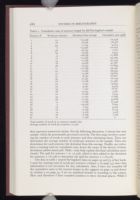
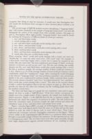
| Sentence # | Words per sentence | Deviation from average | Cumulative sum (qsld) |
| 1 | 12 | −10.258 | −10.258 |
| 2 | 16 | −6.258 | −16.516 |
| 3 | 34 | 11.742 | −4.774 |
| 4 | 7 | −15.258 | −20.032 |
| 5 | 46 | 23.742 | 3.710 |
| 6 | 19 | −3.258 | 0.452 |
| 7 | 4 | −18.258 | −17.806 |
| 8 | 10 | −12.258 | −30.065 |
| 9 | 15 | −7.258 | −37.323 |
| 10 | 18 | −4.258 | −41.581 |
| 11 | 36 | 13.742 | −27.839 |
| 12 | 11 | −11.258 | −39.097 |
| 13 | 22 | −0.258 | −39.355 |
| 14 | 22 | −0.258 | −39.613 |
| 15 | 31 | 8.742 | −30.871 |
| 16 | 33 | 10.742 | −20.129 |
| 17 | 20 | −2.258 | −22.387 |
| 18 | 25 | 2.742 | −19.645 |
| 19 | 32 | 9.742 | −9.903 |
| 20 | 24 | 1.742 | −8.161 |
| 21 | 36 | 13.742 | 5.581 |
| 22 | 22 | −0.258 | 5.323 |
| 23 | 34 | 11.742 | 17.065 |
| 24 | 40 | 17.742 | 34.806 |
| 25 | 15 | −7.258 | 27.548 |
| 26 | 3 | −19.258 | 8.290 |
| 27 | 23 | 0.742 | 9.032 |
| 28 | 20 | −2.258 | 6.774 |
| 29 | 19 | −3.258 | 3.516 |
| 30 | 20 | −2.258 | 1.258 |
| 31 | 21 | −1.258 | 0 |
Total number of words in 31-sentence sample: 690
Average number of words per sentence: 22.258
that represent numerical entities. For the following discussion, I choose her own
sample, which she presumably processed correctly. The first stage involves
count-
ing the number of words in each sentence and then tabulating them.
Then one
determines the average number of words per sentence in the sample.
Then one
determines for each sentence the deviation from this average.
Finally, one calcu-
lates a running total (or cumulative sum, hence the name
of the theory) of these
deviations (abbreviated qsld). Table 1 may help explain this final calculation more
clearly.
The qsld for sentence 1 is −10.258, which is then added to the deviation
for sentence 2 (−6.258) to determine the qsld for sentence 2
(−16.516).
The data in table 1 match Farringdon's data on pages 33 and 55 of her book.
I omit the running total of words per sentence (column 2 on page 55) since that
information is not necessary for any calculation. Also, I have not rounded
off
the cumulative sums to the nearest integer as she suggests on page 19
and shows
in column 5 on page 55. I see no statistical benefit to rounding
to this extent.
Here and elsewhere I have rounded numbers to three decimal
places. While I
self rounds the deviations from averages to three decimal places (column 4 on
page 55).
The second stage of QSUM analysis involves identifying a "language-habit"
that "will remain consistent in the sample of language being tested" (19) and will
distinguish the author of the sample from other possible authors. On pages
20
and 25, Farringdon offers eight possible "language-habits" that could be
tested
by counting the frequency of different kinds of words per
sentence:
- 1. two- and three-letter words
- 2. words starting with a vowel
- 3. two- and three-letter words plus words starting with a vowel
- 4. two-, three-, and four-letter words
- 5. two-, three-, and four-letter words plus words starting with a vowel
- 6. three- and four-letter words
- 7. three- and four-letter words plus words starting with a vowel
- 8. words other than two- or three-letter words
When counting "short" words and words starting with a vowel, one must not
"double-dip" or count the same word twice. (The word "and," for example, is
a three-letter word that begins with a vowel, but it cannot be counted as two
words.) She also states that "the most satisfactory percentage of 'habit'
words per
sentence is between 45 and 55 per cent" (25). For her own writing,
she usually
chooses test #3, two- and three-letter words plus words starting
with a vowel.
For this 31-sentence sample, the average number of these words
per sentence is
11.677, which is 52.5% of the average number of total
words per sentence and is
comfortably within her "satisfactory" range. After
counting the words belonging
to the selected "language-habit" one then
performs cumulative sum calculations
similar to the ones conducted for
sentence length. Table 2 presents these results.
The second column is headed
"23lw+ivw," her abbreviation for "two- and three-
letter words plus words
starting with a vowel." The data in the second column
of table 2 match
Farringdon's data in the last column on page 33. (She does not
provide raw
data for the other two columns, but the resulting graph shows that
my
numbers match hers.)
The third and final stage is to graph the two cumulative sums and to super-
impose the lines to make a "QSUM-chart." If the lines closely correspond, the
sample text is by a single author. If they separate, the sample text results
from a
mixed utterance. Figure 1 is the QSUM-chart for the 31-sentence
sample. The
horizontal axis charts the sequence of sentences in order. The
left vertical axis
charts the cumulative sums of sentence length; the right
vertical axis charts the
cumulative sums of two- and three-letter and
initial-vowel words.
Figure 1 matches figure JMF-3 on page 36 of Farringdon's book. This would
make sense since both figures derive from the same set of data and use the same
method to scale the chart (I discuss scale in more detail later). Thus I
have
replicated the technique correctly. Farringdon comments on this figure:
"What
is here visible in the superimposed QSUM-chart is a consistent habit
running
through a reasonable sample of thirty-one sentences. To the
experienced eye, this
is a homogeneous chart. The two lines track each other
quite smoothly, though
some slight displacement appears around sentences
18–20, resulting in what
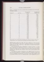
| Sentence # | 23lw+ivw | Deviation from average |
Cumulative sum (qs23lw+ivw) |
| 1 | 5 | −6.677 | −6.677 |
| 2 | 12 | 0.323 | −6.355 |
| 3 | 17 | 5.323 | −1.032 |
| 4 | 5 | −6.677 | −7.710 |
| 5 | 25 | 13.323 | 5.613 |
| 6 | 7 | −4.677 | 0.935 |
| 7 | 1 | −10.677 | −9.742 |
| 8 | 4 | −7.677 | −17.419 |
| 9 | 7 | −4.677 | −22.097 |
| 10 | 9 | −2.677 | −24.774 |
| 11 | 21 | 9.323 | −15.452 |
| 12 | 6 | −5.677 | −21.129 |
| 13 | 12 | 0.323 | −20.806 |
| 14 | 11 | −0.677 | −21.484 |
| 15 | 15 | 3.323 | −18.161 |
| 16 | 17 | 5.323 | −12.839 |
| 17 | 13 | 1.323 | −11.516 |
| 18 | 16 | 4.323 | −7.194 |
| 19 | 17 | 5.323 | −1.871 |
| 20 | 15 | 3.323 | 1.452 |
| 21 | 14 | 2.323 | 3.774 |
| 22 | 10 | −1.677 | 2.097 |
| 23 | 19 | 7.323 | 9.419 |
| 24 | 23 | 11.323 | 20.742 |
| 25 | 9 | −2.677 | 18.065 |
| 26 | 2 | −9.677 | 8.387 |
| 27 | 10 | −1.677 | 6.710 |
| 28 | 10 | −1.677 | 5.032 |
| 29 | 8 | −3.677 | 1.355 |
| 30 | 11 | −0.677 | 0.677 |
| 31 | 11 | −0.677 | 0 |
Total number of two- and three-letter and initial-vowel words in 31-sentence sample: 362
Average number of two- and three-letter and initial vowel-words per sentence: 11.677
QSUM-analysts usually call a 'blip': this may be defined as a minor and tem-
porary visual disturbance rather than a continuing separation" (37). Farringdon
explains that the "blip" results from a "high degree of condensed
information"
(37) in sentences 18–20.
I have presented this primer of QSUM for a number of reasons: 1) to show
that I understand the mathematics involved; 2) to show that I can accurately
replicate the method; and 3) to establish a basis upon which I will analyze
further
examples more efficiently. First, though, I want to raise central
questions about
this method.
I can think of a number of objections to the QSUM method. The lack of
any
theoretical justification is troubling, and leaves the skeptical outsider with
no way to challenge the proponents on this basis. I suspect that a linguist
would
be especially dubious, since the "language-habits" used in QSUM do not
cor-
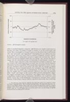

FIGURE 1. Jill Farringdon's sample.
function, but rather according to length or whether or not the words begin with
vowels. How meaningful is a category (such as test #3 above) that would include
"the" and "anaconda" and "apprehend"? Farringdon does not address this issue
in any detail, and in her book I find no citations of linguistic research. Indeed,
Farringdon cites no independent research to support her assertion that "the use
of these unconscious linguistic habits does not change" (84), and she thus fails to
engage with the substantial amount of scholarship on intra-speaker variation.[7]
Another major objection is that visual inspection of charts is imprecise. And
one wonders why visual inspection is necessary since all of the relevant
linguistic
information has been quantified. Why not develop a quantitative
scheme to com-
pare the cumulative sums at every point? The chart, after
all, attempts to display
the difference (shown vertically) between the
cumulative sums. If the differences
are small, then the sample text is
homogeneous. If the differences are large,
then the sample text is a mixed
utterance. However, how does one precisely
define "small" and "large" in
this context? What precisely distinguishes "blips"
that suggest anomalies
from "separations" that suggest mixed utterance? With
a quantitative method
and the consequent calculations, one would then need
specific criteria that
would distinguish a homogeneous utterance from a mixed
utterance. If all of
these criteria could be expressed numerically, that would help
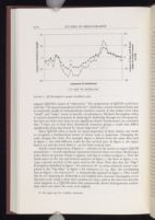

FIGURE 2. Jill Farringdon's sample (modified scale).
used the "chi-squared goodness-of-fit test" which has a sound statistical basis and
is commonly taught in undergraduate statistics courses. It also makes clear what
"small" and "large" mean in specific circumstances. Michael Farringdon refers
to various statistical measures in Analysing for Authorship (though not chi-squared),
but does not delve into them in any significant detail. Furthermore, he concludes
that "I have yet to find these [statistical] measures giving a result that differs
significantly from that found by visual inspection" (261).[8]
Since QSUM relies so much on visual inspection of these charts, one needs
to
recognize a fundamental axiom of charts: scale is important. Changing the
scale changes the chart. For example, figure 2 derives from the same data used
in figure 1, but with different scales for the vertical axes. In figure 2,
the upper
limit is 50 and the lower limit is −50 for both vertical
axes.
Surely, visual inspection of figure 2—whether by the novice or expert QSUM
practitioner—reveals significant separation between these two lines.
Reducing a
scale allows for greater detail to appear, and this is evident in
figure 2. Note the
blank space in the top and bottom quarters of figure 1;
the lines in figure 2 oc-
cupy a greater portion of the space used in the
chart. Note also that the "blips"
Farringdon identified in figure 1 for
sentences 18–20 seem relatively minor com-
pared to the "big blips"
in figure 2 for sentences 12–14. Also, the overlapping
lines in
figure 1 for sentences 6–11 dramatically separate in figure 2. Why would
this be so? Analysing for Authorship is not helpful
here, because Farringdon never
discusses scale using a chart that contains
two lines, and so she does not describe
what happens to a QSUM-chart that
purportedly shows homogeneous author-
ship when one alters the scale even
slightly.
Her brief discussion of scale sets out rules "in order that graphs or charts
may be drawn in a perspective which provides clear information by visual dis-
play" (52). She adds that "the objective is that the graph show the line at
about
one quarter to one third of the vertical range of the sample in
proportion to the
horizontal space" (52). To determine what she defines as
the appropriate scale
for the cumulative sum of sentence length, she first
determines the maximum
and minimum values of this cumulative sum for the
sample chosen. In this in-
stance, the maximum is 34.806 (for sentence 24 in
table 1) and the minimum is
−41.581 (for sentence 10). In this
instance, adding the absolute
values (absolute values ignore the negative
and positive signs) of the maximum and minimum
gives the range, which in
this example is 76.387. Since Farringdon rounds the
cumulative sum for
sentence length to the nearest integer, she finds a range of
77. The
difference is not significant, and so for the purposes of this discussion, I
will treat the range as exactly 77. The scale in figure 1 for the cumulative sum
of sentence length uses 120 as the upper limit and −120 as the lower
limit. The
entire range for this vertical axis is thus 240. If we divide 77
by 240 we get .321,
which is within Farringdon's preference of between one
quarter to one third. In
figure 1, Farringdon's vertical axis on the right
also yields a proportion of .321,
producing almost identical proportions for
the scaling of both vertical axes. The
altered vertical axes in figure 2 use
a range of 100, and the percentages (77/100 =
.77 and 46/100 = .46) are
outside her preference.
Because Farringdon relies solely on a visual impression in relation to the
scale, her method of scaling is arbitrary. (It is also imprecise; "about one
quarter
to one third" allows for enough variation that could significantly
affect the ap-
pearance of the chart.) The arbitrariness of her scaling
method leaves her open
to the charge that she is prejudicial toward the
presentation of her data, as her
method allows her to determine the scale
after performing her calculations. What
she needs
is a scaling method that must be set prior to her
calculations.
To avoid the charge of being arbitrary (and potentially prejudicial), she could
have adopted a standardized scale based on the standard deviation of the
cumu-
lative sums. To create this standardized scale, one would subtract the
mean from
each cumulative sum and divide the difference by the standard
deviation. Figure 3
displays the same data using a standardized scale. This
method requires only
one vertical axis for both lines. This method also
eliminates the arbitrary nature
of her method of scaling. However, the
interpretation of the chart based on a
standardized scale is open to debate.
Does figure 3 reveal that the sample is of
homogeneous or mixed utterance?
The lines overlap for most of the chart, and
the most significant separation
occurs between sentences 17 and 21. Is that sepa-
ration significant? The
separation in figure 3 for those sentences looks greater
than that in figure
1, but it is not clear whether the separation in either figure
is
significant.
So there exists a reliable and consistent way to determine scale that Far-
ringdon could have used. The use of a standardized scale would have removed
any suspicion that she might be manipulating the scale to create charts that skew
her data. However, I cannot determine whether or not she manipulates the
scale
in her book or her recent SB article because
she does not offer the raw data that
provide the basis for her charts. Had
she provided such information she could
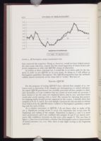

FIGURE 3. Jill Farringdon's sample (standardized scale).
the other main objection, namely that the visual inspection of charts invites sub-
jective judgments at odds with QSUM's claims of objectivity.
As serious as these criticisms are, I would like to set them aside for the mo-
ment in order to test QSUM on its own terms. In doing so, I will adhere to
Farringdon's guidelines throughout. The QSUM proponents base the method's
validity almost exclusively on the claim that it "works." But does it?
Cardiff: Univ. of Wales Press, 1996. This book was favorably reviewed by
Peter Smith
in Forensic Linguistics 5 (1998):
77–79, by Kathryn Summers in D. H. Lawrence
Review 28.1–2
(1999): 182–184, and by Warren
Buckland in The Semiotic Review of Books 10.3 (1999):
10–12,
and negatively reviewed by George K. Barr in Expert Evidence 6 (1998): 43–55 and by Pieter
de Haan in Forensic Linguistics 5 (1998):
69–76. For a concise presentation of QSUM, go to the
author's
website at
<http://members.aol.com/qsums/QsumIntroduction.html>.
Kathryn Lindskoog, Sleuthing C. S. Lewis: More Light in
the Shadowlands (Macon, Georgia:
Mercer Univ. Press, 2001),
262–264.
Eighteenth-Century Fiction 8 (1995–96):
533–538. The quotation occurs on page 537.
Battestin's essay is
part of a forum on attribution prompted by J. Paul Hunter's favorable review
of P. N. Furbank and W. R. Owens, Defoe
De-Attributions: A Critique of J. R. Moore's "Checklist"
in Eighteenth-Century Fiction 8
(1995–96): 310–312. Further contributions by Hunter, Isobel
Grundy, Melvyn New, Hugh Amory, Maximillian E. Novak, Carolyn
Woodward, Barbara
Laning Fitzpatrick, and Furbank and Owens appear in
Eighteenth-Century Fiction 8 (1995–96):
519–538; 9 (1996–97): 89–100, 223–225.
Since I cite Battestin here, I want to be clear: QSUM does not play any part in his edition
of New
Essays by Henry Fielding: His Contributions to the Craftsman (1734–1739) and Other Early
Journalism
(Charlottesville: Univ. Press of Virginia, 1989). That volume contains a
"stylometric
analysis" by Michael Farringdon, but this analysis
differs from QSUM, and so my remarks here
do not directly pertain to
the conclusions reached in those attributions, which I have not exam-
ined in any detail. In Analysing for Authorship, Jill
Farringdon promises that "in due course, all
forty-one of the New Essays [attributed to Fielding] will be analysed
by QSUM, and the results
published" (175). I am not aware of any
publication along these lines.
The following article directly challenges the claim that authors are
consistent in their
use of these "language-habits": Pieter de Haan and
Erik Schils, "The Qsum Plot Exposed," Cre-
ating and
Using English Language Corpora: Papers from the Fourteenth International
Conference on English
Language Corpora, Zürich, 1993,
ed. Udo Fries, Gunnel Tottie, and Peter Schneider (Amsterdam:
Rodopi,
1994), 93–105. Farringdon does not cite this article, and to my
knowledge the QSUM
proponents have not addressed its criticisms.
Testing QSUM
For the purposes of testing QSUM I have selected four samples of 31 sen-
tences each to determine if the samples are homogeneous or mixed utterance.
An expert QSUM practitioner has carefully processed all four samples to elimi-
nate anomalies, so I am confident that my counts of word totals are
accurate. I
have chosen to use the same test employed above, that is, two-
and three-letter
words plus words starting with a vowel. My reasons for
selecting this particu-
lar language-habit should become apparent in due
course. I identify these four
samples as W, X, Y, and Z. For each sample, I
present the relevant data in tabular
form followed by the QSUM-charts. I
adhere to Farringdon's guidelines regard-
ing scale for each of them.
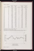
As a relative newcomer to QSUM, I do not know what to make of fig-
ure 4.
Significant overlap seems to occur, but separation also occurs near the
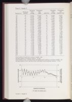
beginning and ending of the sample. Separation in figures 5 and 6 is much
more pronounced, and I am confident that samples X and Y are mixed utter-
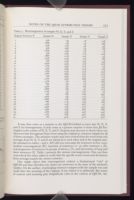
ances. My confidence increases on this score with sample Z. The two lines in
figure 7 criss-cross several times, a feature that Farringdon notes is
characteristic
of mixed utterance (70, 217). Also, there is only slight
overlap at the beginning
and end.
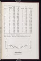
| Sentence # | Words per sentence |
Deviation from average |
Cumulative sum (qsld) |
23lw+ivw | Deviation from average |
Cumulative sum (qs23lw+ivw) |
| 1W | 21 | −1.258 | −1.258 | 11 | −0.677 | −0.677 |
| 2W | 31 | 8.742 | 7.484 | 15 | 3.323 | 2.645 |
| 3W | 12 | −10.258 | −2.774 | 5 | −6.677 | −4.032 |
| 4W | 22 | −0.258 | −3.032 | 10 | −1.677 | −5.710 |
| 5W | 19 | −3.258 | −6.290 | 7 | −4.677 | −10.387 |
| 6W | 25 | 2.742 | −3.548 | 16 | 4.323 | −6.065 |
| 7W | 15 | −7.258 | −10.806 | 7 | −4.677 | −10.742 |
| 8W | 15 | −7.258 | −18.065 | 9 | −2.677 | −13.419 |
| 9W | 7 | −15.258 | −33.323 | 5 | −6.677 | −20.097 |
| 10W | 19 | −3.258 | −36.581 | 8 | −3.677 | −23.774 |
| 11W | 36 | 13.742 | −22.839 | 21 | 9.323 | −14.452 |
| 12W | 34 | 11.742 | −11.097 | 17 | 5.323 | −9.129 |
| 13W | 3 | −19.258 | −30.355 | 2 | −9.677 | −18.806 |
| 14W | 11 | −11.258 | −41.613 | 6 | −5.677 | −24.484 |
| 15W | 22 | −0.258 | −41.871 | 12 | 0.323 | −24.161 |
| 16W | 16 | −6.258 | −48.129 | 12 | 0.323 | −23.839 |
| 17W | 20 | −2.258 | −50.387 | 11 | −0.677 | −24.516 |
| 18W | 4 | −18.258 | −68.645 | 1 | −10.677 | −35.194 |
| 19W | 20 | −2.258 | −70.903 | 10 | −1.677 | −36.871 |
| 20W | 46 | 23.742 | −47.161 | 25 | 13.323 | −23.548 |
| 21W | 36 | 13.742 | −33.419 | 14 | 2.323 | −21.226 |
| 22W | 22 | −0.258 | −33.677 | 11 | −0.677 | −21.903 |
| 23W | 32 | 9.742 | −23.935 | 17 | 5.323 | −16.581 |
| 24W | 23 | 0.742 | −23.194 | 10 | −1.677 | −18.258 |
| 25W | 10 | −12.258 | −35.452 | 4 | −7.677 | −25.935 |
| 26W | 40 | 17.742 | −17.710 | 23 | 11.323 | −14.613 |
| 27W | 33 | 10.742 | −6.968 | 17 | 5.323 | −9.290 |
| 28W | 24 | 1.742 | −5.226 | 15 | 3.323 | −5.968 |
| 29W | 18 | −4.258 | −9.484 | 9 | −2.677 | −8.645 |
| 30W | 34 | 11.742 | 2.258 | 19 | 7.323 | −1.323 |
| 31W | 20 | −2.258 | 0 | 13 | 1.323 | 0 |
Total number of words in 31-sentence sample: 690
Average number of words per sentence: 22.258
Total number of two- and three-letter and initial-vowel words in 31-sentence sample: 362
Average number of two- and three-letter and initial vowel-words per sentence: 11.677

FIGURE 4. Sample W.
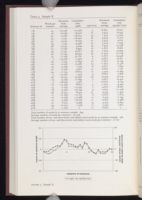
| Sentence # | Words per sentence |
Deviation from average |
Cumulative sum (qsld) |
23lw+ivw | Deviation from average |
Cumulative sum (qs23lw+ivw) |
| 1X | 12 | −10.258 | −10.258 | 5 | −6.677 | −6.677 |
| 2X | 16 | −6.258 | −16.516 | 12 | 0.323 | −6.355 |
| 3X | 20 | −2.258 | −18.774 | 13 | 1.323 | −5.032 |
| 4X | 25 | 2.742 | −16.032 | 16 | 4.323 | −0.710 |
| 5X | 32 | 9.742 | −6.290 | 17 | 5.323 | 4.613 |
| 6X | 24 | 1.742 | −4.548 | 15 | 3.323 | 7.935 |
| 7X | 36 | 13.742 | 9.194 | 14 | 2.323 | 10.258 |
| 8X | 22 | −0.258 | 8.935 | 10 | −1.677 | 8.581 |
| 9X | 34 | 11.742 | 20.677 | 19 | 7.323 | 15.903 |
| 10X | 40 | 17.742 | 38.419 | 23 | 11.323 | 27.226 |
| 11X | 15 | −7.258 | 31.161 | 9 | −2.677 | 24.548 |
| 12X | 3 | −19.258 | 11.903 | 2 | −9.677 | 14.871 |
| 13X | 23 | 0.742 | 12.645 | 10 | −1.677 | 13.194 |
| 14X | 20 | −2.258 | 10.387 | 10 | −1.677 | 11.516 |
| 15X | 19 | −3.258 | 7.129 | 8 | −3.677 | 7.839 |
| 16X | 20 | −2.258 | 4.871 | 11 | −0.677 | 7.161 |
| 17X | 34 | 11.742 | 16.613 | 17 | 5.323 | 12.484 |
| 18X | 7 | −15.258 | 1.355 | 5 | −6.677 | 5.806 |
| 19X | 46 | 23.742 | 25 097 | 25 | 13.323 | 19.129 |
| 20X | 19 | −3.258 | 21.839 | 7 | −4.677 | 14.452 |
| 21X | 4 | −18.258 | 3.581 | 1 | −10.677 | 3.774 |
| 22X | 10 | −12.258 | −8.677 | 4 | 7.677 | 3.903 |
| 23X | 15 | −7.258 | −15.935 | 7 | −4.677 | −8.581 |
| 24X | 18 | −4.258 | −20.194 | 9 | −2.677 | −11.258 |
| 25X | 36 | 13.742 | −6.452 | 21 | 9.323 | −1.935 |
| 26X | 11 | −11.258 | −17.710 | 6 | −5.677 | −7.613 |
| 27X | 22 | −0.258 | −17.968 | 12 | 0.323 | −7.290 |
| 28X | 22 | −0.258 | −18.226 | 11 | −0.677 | −7.968 |
| 29X | 31 | 8.742 | −9.484 | 15 | 3.323 | −4.645 |
| 30X | 33 | 10.742 | 1.258 | 17 | 5.323 | 0.677 |
| 31X | 21 | −1.258 | 0 | 11 | −0.677 | 0 |
Total number of words in 31 -sentence sample: 690
Average number of words per sentence: 22.258
Total number of two- and three-letter and initial-vowel words in 31-sentence sample: 362
Average number of two- and three-letter and initial vowel-words per sentence: 11.677

FIGURE 5. Sample X.
| Sentence # | Words per sentence |
Deviation from average |
Cumulative sum (qsld) |
23lw+ivw | Deviation from average |
Cumulative sum (qs23lw+ivw) |
| 1Y | 12 | −10.258 | −10.258 | 5 | −6.677 | −6.677 |
| 2Y | 16 | −6.258 | −16.516 | 12 | 0.323 | −6.355 |
| 3Y | 34 | 11.742 | −4.774 | 17 | 5.323 | −1.032 |
| 4Y | 7 | −15.258 | −20.032 | 5 | −6.677 | −7.710 |
| 5Y | 46 | 23.742 | 3.710 | 25 | 13.323 | 5.613 |
| 6Y | 20 | −2.258 | 1.452 | 13 | 1.323 | 6.935 |
| 7Y | 25 | 2.742 | 4.194 | 16 | 4.323 | 11.258 |
| 8Y | 32 | 9.742 | 13.935 | 17 | 5.323 | 16.581 |
| 9Y | 24 | 1.742 | 15.677 | 15 | 3.323 | 19.903 |
| 10Y | 36 | 13.742 | 29.419 | 14 | 2.323 | 22.226 |
| 11Y | 19 | −3.258 | 26.161 | 7 | −4.677 | 17.548 |
| 12Y | 4 | −18.258 | 7.903 | 1 | −10.677 | 6.871 |
| 13Y | 10 | −12.258 | −4.355 | 4 | −7.677 | −0.806 |
| 14Y | 15 | −7.258 | −11.613 | 7 | −4.677 | −5.484 |
| 15Y | 18 | −4.258 | −15.871 | 9 | −2.677 | −8.161 |
| 16Y | 22 | −0.258 | −16.129 | 10 | −1.677 | −9839 |
| 17y | 34 | 11.742 | −4.387 | 19 | 7.323 | −2.516 |
| 18Y | 40 | 17.742 | 13.355 | 23 | 11.323 | 8.806 |
| 19Y | 15 | −7.258 | 6.097 | 9 | −2.677 | 6.129 |
| 20Y | 3 | −19.258 | −13.161 | 2 | −9.677 | −3.548 |
| 21Y | 36 | 13.742 | 0.581 | 21 | 9.323 | 5.774 |
| 22Y | 11 | −11.258 | −10.677 | 6 | −5.677 | 0.097 |
| 23Y | 22 | −0.258 | −10.935 | 12 | 0.323 | 0.419 |
| 24Y | 22 | −0.258 | −11.194 | 11 | −0.677 | −0.258 |
| 25Y | 31 | 8.742 | −2.452 | 15 | 3.323 | 3.065 |
| 26Y | 33 | 10.742 | 8.290 | 17 | 5.323 | 8.387 |
| 27Y | 23 | 0.742 | 9.032 | 10 | −1.677 | 6.710 |
| 28Y | 20 | −2.258 | 6.774 | 10 | −1.677 | 5.032 |
| 29Y | 19 | −3.258 | 3.516 | 8 | −3.677 | 1.355 |
| 30Y | 20 | −2.258 | 1.258 | 11 | −0.677 | 0.677 |
| 31Y | 21 | −1.258 | 0 | 11 | −0.677 | 0 |
Total number of words in 31 -sentence sample: 690
Average number of words per sentence: 22.258
Total number of two- and three-letter and initial-vowel words in 31 -sentence sample: 362
Average number of two- and three-letter and initial vowel-words per sentence: 11.677

FIGURE 6. Sample Y.
| Sentence # | Words per sentence |
Deviation from average |
Cumulative sum (qsld) |
23lw+ivw | Deviation from average |
Cumulative sum (qs23lw+ivw) |
| 1Z | 46 | 23.742 | 23.742 | 25 | 13.323 | 13.323 |
| 2Z | 3 | −19.258 | 4.484 | 2 | −9.677 | 3.645 |
| 3Z | 40 | 17.742 | 22.226 | 23 | 11.323 | 14.968 |
| 4Z | 4 | −18.258 | 3.968 | 1 | −10.677 | 4.290 |
| 5Z | 36 | 13.742 | 17.710 | 21 | 9.323 | 13.613 |
| 6Z | 7 | −15.258 | 2.452 | 5 | −6.677 | 6.935 |
| 7Z | 36 | 13.742 | 16.194 | 14 | 2.323 | 9.258 |
| 8Z | 10 | −12.258 | 3.935 | 4 | −7.677 | 1.581 |
| 9Z | 34 | 11.742 | 15.677 | 17 | 5.323 | 6.903 |
| 10Z | 11 | −11.258 | 4.419 | 6 | −5.677 | 1.226 |
| 11Z | 34 | 11.742 | 16.161 | 19 | 7.323 | 8.548 |
| 12Z | 12 | −10.258 | 5.903 | 5 | −6.677 | 1.871 |
| 13Z | 33 | 10.742 | 16.645 | 17 | 5.323 | 7.194 |
| 14Z | 15 | −7.258 | 9.387 | 7 | −4.677 | 2.516 |
| 15Z | 32 | 9.742 | 19.129 | 17 | 5.323 | 7.839 |
| 16Z | 15 | −7.258 | 11.871 | 9 | −2.677 | 5.161 |
| 17Z | 31 | 8.742 | 20.613 | 15 | 3.323 | 8.484 |
| 18Z | 16 | −6.258 | 14.355 | 12 | 0.323 | 8.806 |
| 19Z | 25 | 2.742 | 17.097 | 16 | 4.323 | 13.129 |
| 20Z | 18 | −4.258 | 12.839 | 9 | −2.677 | 10.452 |
| 21Z | 24 | 1.742 | 14.581 | 15 | 3.323 | 13.774 |
| 22Z | 19 | −3.258 | 11.323 | 7 | −4.677 | 9.097 |
| 23Z | 23 | 0.742 | 12.065 | 10 | −1.677 | 7.419 |
| 24Z | 19 | −3.258 | 8.806 | 8 | −3.677 | 3.742 |
| 25Z | 22 | −0.258 | 8.548 | 12 | 0.323 | 4.065 |
| 26Z | 20 | −2.258 | 6.290 | 13 | 1.323 | 5.387 |
| 27Z | 22 | −0.258 | 6.032 | 11 | −0.677 | 4.710 |
| 28Z | 20 | −2.258 | 3.774 | 10 | −1.677 | 3.032 |
| 29Z | 22 | −0.258 | 3.516 | 10 | −1.677 | 1.355 |
| 30Z | 20 | −2.258 | 1.258 | 11 | −0.677 | 0.677 |
| 31Z | 21 | −1.258 | 0 | 11 | −0.677 | 0 |
Total number of words in 31-sentence sample: 690
Average number of words per sentence: 22.258
Total number of two- and three-letter and initial-vowel words in 31-sentence sample: 362
Average number of two- and three-letter and initial vowel-words per sentence: II.677

FIGURE 7. Sample Z.
| Original Sentence # | Sample W | Sample X | Sample Y | Sample Z |
| 1 | 3W | 1X | 1Y | 12Z |
| 2 | 16W | 2X | 2Y | 18Z |
| 3 | 12W | 17X | 3Y | 9Z |
| 4 | 9W | 18X | 4Y | 6Z |
| 5 | 20W | 19X | 5Y | 1Z |
| 6 | 5W | 20X | 11Y | 22Z |
| 7 | 18W | 21X | 12Y | 4Z |
| 8 | 25W | 22X | 13Y | 8Z |
| 9 | 7W | 23X | 14Y | 14Z |
| 10 | 29W | 24X | 15Y | 20Z |
| 11 | 11W | 25X | 21Y | 5Z |
| 12 | 14W | 26X | 22Y | 10Z |
| 13 | 15W | 27X | 23Y | 25Z |
| 14 | 22W | 28X | 24Y | 27Z |
| 15 | 2W | 29X | 25Y | 17Z |
| 16 | 27W | 30X | 26Y | 13Z |
| 17 | 31W | 3X | 6Y | 26Z |
| 18 | 6W | 4X | 7Y | 19Z |
| 19 | 23W | 5X | 8Y | 15Z |
| 20 | 28W | 6X | 9Y | 21Z |
| 21 | 21W | 7X | 10Y | 7Z |
| 22 | 4W | 8X | 16Y | 29Z |
| 23 | 30W | 9X | 17Y | 11Z |
| 24 | 26W | 10X | 18Y | 3Z |
| 25 | 8W | 11X | 19Y | 16Z |
| 26 | 13W | 12X | 20Y | 2Z |
| 27 | 24W | 13X | 27Y | 23Z |
| 28 | 19W | 14X | 28Y | 28Z |
| 29 | 10W | 15X | 29Y | 24Z |
| 30 | 17W | 16X | 30Y | 30Z |
| 31 | 1W | 31X | 31Y | 31Z |
It may thus come as a surprise to the QSUM faithful to learn that W, X, Y,
and Z are homogeneous. It may come as a greater surprise to learn that Jill Far-
ringdon is the author of W, X, Y, and Z. Surprise may increase to shock when
one
discovers that throughout I have been using the original 31-sentence
sample for all
of these examples. The attentive reader may have noticed that
the word totals and
averages from W, X, Y, and Z are identical to each other
and to the original sam-
ple tabulated in tables 1 and 2. All I did was
rearrange the sentences in four ways:
random rearrangement (W), insertion of
sentences 17–30 after sentence 2 (X),
rearrangement of sentences in
groups of about 5 (Y), and alternation of long and
short sentences (Z).
Table 7 presents the various rearrangements. One can then
cross-check the
other tables to verify that the specific word counts and deviations
from
averages match the correct sentence.
One might object that rearrangement violates a fundamental "rule" of
QSUM
and that therefore my charts are irrelevant to the issue of the method's
validity. On the surface, rearranging sentences tampers with the sample text and
could alter the meaning of the original, if not reduce it to gibberish. But
issues
of content and meaning play insignificant roles in the context of
QSUM. Ad-
I performed what Farringdon calls a "sandwich": "A 'sandwich' is a useful test:
as its name indicates, it is a procedure whereby a new sample of sentences is
inserted into utterance already tested and found to be homogeneous" (305n14).
Indeed, she often uses this test. In the case of sample X, I did not insert a "new"
sample, but then again, all the sentences here were purported to be "already
tested and found to be homogeneous." Sample X produced figure 5, which ac-
cording to QSUM clearly indicates mixed utterance—even more so than the
random version I call sample W, which produced figure 4. On the issue of ran-
dom rearrangement, Farringdon writes: "It has been pointed out by members of
an academic audience on different occasions that sentences in various QSUM
examples displayed need not be sequential, and that they would produce the
same consistency if analysed in random order. This is true" (114). Elsewhere, Far-
ringdon recommends alternating short samples: "This can be done by following
a small number of sentences (between four to eight) of one author with a similar
number of the second author, until your sample is completely used up" (120). I
used this method to create sample Y, which produced figure 6. For sample Z, I
intended to create a "roller-coaster" effect, such that the alternation of longest
and shortest sentences would bounce the lines up and down. Doing so causes
definite separation in this instance.
How can this be? The answer returns us to the fundamental nature of QSUM
which is evident in its name: cumulative sums. Despite Farringdon's assurances to
the contrary, sequence order matters greatly when calculating cumulative
sums.
Table 7 compares the relevant data for any particular sentence
generated for the
original sample, W, X, Y, and Z. One can quickly tell that
no matter how the
sentences are rearranged, certain information does not
change. The cumulative
sums, however, almost always change. Table 8 uses
sentence 10 of the original
sample and its equivalents as an example.
Obviously, the number of words per sentence will not change no matter
where
that sentence has been rearranged in the sample. Also, the number of
types
of words (in this case, two- and three-letter words and words beginning
with
a vowel) will not change. And since the contents of the entire sample have
not been altered, the averages will remain the same, and therefore the deviations
from those averages will also stay constant. The cumulative sums, however,
de-
pend on the previous cumulative sums, which depend on the previous
cumulative
sums, etc. Anyone who has even a basic familiarity with
statistics would know
that altering the sequence almost always changes the
cumulative sums. The im-
plications of this fact are devastating for the
theory called QSUM. This should
already be apparent when comparing figures
1, 4, 5, 6, and 7 and recognizing
that they display radically different
QSUM-charts for the same utterance. Con-
trary to Farringdon's assertions,
the order of the sequence matters a great deal.
Thus one must wonder why the proponents use cumulative sums. I find no
theoretical explanation of this approach in Analysing for
Authorship beyond a pass-
ing reference to the method's origins:
"Morton first suggested the idea of cumu-
lative sum tests for language as
long ago as the 1960s, carrying the idea over
from its industrial setting:
such tests are widely used in industry as a method of
sampling averages"
(13). Farringdon is correct on this point; cumulative sums are
| Sentence # | Words per sentence |
Deviation from average |
Cumulative sum (qsld) |
23lw+ivw | Deviation from average |
Cumulative sum (qs23lw+ivw) |
| 10 | 18 | −4.258 | −41.581 | 9 | −2.677 | −24.774 |
| 29W | 18 | −4.258 | −9.484 | 9 | −2.677 | −8.645 |
| 24X | 18 | −4.258 | −20.194 | 9 | −2.677 | −11.258 |
| 15Y | 18 | −4.258 | −15.871 | 9 | −2.677 | −8.161 |
| 20Z | 18 | −4.258 | 12.839 | 9 | −2.677 | 10.452 |
useful for those who want to detect slight deviations from the mean in a
particular
process over time (i. e., in a time-increasing sequence). For
example, engineers
involved with quality control find this technique
useful.[9]
Morton, Farringdon, and others thus adapt a reliable statistical technique for
purposes that have nothing whatever to do with the technique's original
func-
tion. That in itself is not a problem, for many statistical techniques
find valid
uses beyond their original applications. But the uses are valid
only when the
proponents are using the techniques to measure phenomena that
are demonstra-
bly analogous. The burden falls on Farringdon and her
associates to show that
cumulative sum analysis is applicable for
determining the authorship of texts.
What analogies exist between quality
control and the attribution of authorship?
Those involved with quality
control want to know how change occurs during a
particular sequence, and so
they would never rearrange the data in the way that
I have done (and as
recommended by Farringdon). Those involved with attribu-
tion want to know
how particular linguistic features distinguish one author from
another. Such
interests in the use of language have nothing to do with sequence
or with
change, which is presumably why Farringdon believes that "sentences
in
various QSUM examples displayed need not be sequential" (114). Attribution
study—even the branch of attribution study concerned with
quantitatively-based
theories—does not generally explore the sequence
of the sentences. And even if
the sequence of the sentences was a topic of
interest, one would have to expect
that the text's final sequence would
often differ greatly from the sequence of
earlier versions; most authors cut
and paste. By rearranging sets of sentences in
the way that Farringdon has
done, she has misused the technique of cumulative
sums and has applied it
for purposes that have nothing to do with the original
technique.
In addition, cumulative sums as used in quality control measure one variable.
As far as I can tell, cumulative sum charts never compare multiple variables.
In this context, it
is worth pointing out that in Analysing for Authorship, the
Far-
ringdons favorably refer to the work of A. F. Bissell, who has
published on the
use of cumulative sum charts for various industrial
applications. In the article
of which contain only one variable each.[10] If I am correct that these charts never
compare multiple variables—and this issue is never addressed in Analysing for
Authorship—then Morton and Farringdon have drastically altered and mishan-
dled a valid statistical technique.
What are possible objections to these criticisms? Every one that I can think
of would apply equally to the QSUM proponents. My sample text was processed
by Jill Farringdon herself. The sample was examined using the "language-habit"
test that she identified as reliably distinguishing her utterance from that
of oth-
ers. The methods of combining different sets of sample texts are
based on Far-
ringdon's guidelines. The formulas for scaling each vertical
axis are also based on
her guidelines. Nonetheless, the four charts for
samples W, X, Y, and Z dramati-
cally differ from the one Farringdon
presents, even though all the charts derive
from the same raw data. Using
the techniques outlined here, anyone could re-
peat this falsification
process for almost any set of data provided by QSUM
proponents.
Perhaps the only objection available to the QSUM proponents is that I did
not use the transparency method that Farringdon recommends as preferable to
the charts: "the more sensitive way to compare the sentence-length and habit
is to print out separate graphs for each, and to compare the movement of the
sentence and habit deviations by the use of transparencies. Indeed, this method
is essential for any serious project, and is the
proper method for isolating either
single-sentence anomalies or aberrant
interpolations of passages which typically
constitute mixed utterance" (35).
The transparency method, however, is more
subjective than the charts. With
the charts, different examiners can at least agree
on the visual data being
displayed; transparencies would add ambiguity and raise
questions about how
one should manipulate the graphs. How does one overlay
one graph upon
another? Are the initial points and/or the terminal points se-
lected as
fixed positions of reference? Doing so will probably result in something
nearly identical to the QSUM-charts presented here and in Farringdon's book.
Can one adjust the superimposed graphs in any way? Farringdon does not say,
and her language on this crucial point is remarkably vague.
Elsewhere Farringdon writes that once one has these separate graphs on
transparencies one then needs "to see whether the two graph-lines track each
other closely, or even coincide."[11]
What exactly does "track" mean? Again,
Farringdon does not clarify
this term, as if its meaning were obvious. One in-
terpretation could be
that the lines track each other when they have a similar
shape, though this
too is vague. But this general issue should return us to the
fundamental
matter of exactly what linguistic information QSUM purports to
when above average information is displayed, and downward when below aver-
age information is displayed. Or, to take the example of sentence length (qsld),
the line will move upward for a longer than average sentence and downward for
a shorter than average sentence. (This average is determined by the sample under
examination.) This principle also holds for the line representing the language-
habit being used. If one is measuring the number of two- and three-letter and
initial-vowel words, then the line moves upward or downward depending on the
deviation from the average number of this class of words per sentence (again,
with the average determined by the sample being studied).
So when these two lines "track" or follow the same shape, they tend to move
up and down at the same points and with similar slopes. If one ignores the issue
of whether or not the lines coincide at any particular point, one can see
that for
figures 1–7, the two lines of each chart follow similar
shapes. In every example
that Farringdon presents, the two lines of each
chart follow similar shapes as
well—regardless of whether or not the
chart purports to establish homogenous
or mixed utterance. These lines
"track" each other quite well because of an
obvious linguistic fact: since
longer sentences, by definition, have more words
(relative to some baseline
of measurement), they will tend to have more words of
a particular class.
And of course a similar principle holds for shorter sentences.
The degree of
this tendency can vary, but will generally hold true. If one can
move the
transparencies when overlaying them, then one could show that the
lines
"track" in almost every instance.
In conclusion, QSUM uses vague definitions for its terms, misuses a valid
statistical technique, and relies on visual inspection without employing a stan-
dardized method for calculating scale. Finally, it does not, in any sense of
the
word, "work." QSUM has no validity. But since an invalid method may well
reach true conclusions, I offer no judgment on the attributions or
de-attributions
that Farringdon presents. Readers should not conclude from my discussion that,
for example, D. H. Lawrence
did indeed write the short story "The Back Road."
Rather, they should
recognize that QSUM does not offer any valid judgment on
this attribution or
on any other. This method is so faulty that one can manipulate
it to claim
any position on any particular attribution.[12]
For a brief discussion of cumulative sums in this context, see Richard A.
Johnson,
Miller and Freund's Probability and Statistics for
Engineers, 7th ed. (Upper Saddle River, New Jer-
sey: Pearson
Prentice Hall, 2005), 525–526. See also the discussion in the Engineering Statistics
Handbook of the U. S.
National Institute of Standards and Technology, located at this website:
<http://www.itl.nist.gov/div898/handbook/pmc/section3/pmc323.htm>.
For references to Bissell, see pages xii, 243, 258–259, and 315n20.
In the final refer-
ence, Michael Farringdon cites the following
article: A. F. Bissell, "Weighted Cusums—Method
and
Applications," Total Quality Management 1.3 (1990):
391–402. In Morton's earlier work, he
presented cumulative sum
charts that contain only one variable: Literary Detection:
How to Prove
Authorship and Fraud in Literature and Documents
(New York: Scribner's, 1978), 78, 81, 84, 85,
and 170.
The following article presents a critical assessment of the QSUM approach
proposed
by A. Q. Morton and S. Michaelson: Michael L. Hilton and
David I. Holmes, "An Assess-
ment of Cumulative Sum Charts for
Authorship Attribution," Literary and Linguistic
Computing 8
(1993): 73–80. The authors offer cogent
criticism, but do not attempt to falsify the technique
in the way that
I do.
Alternatives to Cumulative Sums
Farringdon asserts but does not prove that her "language-habits" help to
distinguish one author from another. As I have already suggested, the assump-
tions behind her method may not have a reliable linguistic basis. But how
can
we know? One could test the hypothesis that Farringdon's
"language-habits"
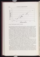

FIGURE 8. Jill Farringdon's sample as scatterplot.
statistical techniques to do so that have nothing to do with cumulative sums.
Farringdon wants to explore the relationship between two variables: the num-
ber of total words per sentence and the number of words in a particular class per
sentence. To display this relationship, one would not use cumulative sum
charts
(which are not used to display the relationship between two
variables), but a scat-
terplot. The scatterplot would use the horizontal
axis for total number of words
per sentence, and the vertical axis for
number of words in a particular class per
sentence. For the following
example, I will use the same class that I have used
throughout, namely two-
and three-letter plus initial-vowel words. Each point on
the scatterplot
represents the data for a single sentence. The scatterplot also helps
to
avoid the problem of sequence that plagues QSUM, since the rearrangement
of
sentences in the sample will not change the appearance of the scatterplot.
Figure 8 is a scatterplot for Farringdon's 31-sentence sample.
One can immediately tell certain things about the relationship between the
two variables. First, one can see that longer sentences tend to have more two- and
three-letter plus initial-vowel words. (As I have already shown, this is not
in any
way a surprise.) Statisticians would call this a positive
association. The relation-
ship also seems to be linear, since the points
tend to cluster around an imaginary
line. Statisticians would also state
that this relationship seems to be particularly
strong, since the points lie
relatively close to this line with little "scatter."
Since the relationship appears linear, we could draw a line through these
points. Obviously, we would like to draw the best possible line, and the "least-
squares regression line" meets this demand in the sense of minimizing the
error in
predicting the number of two- and three-letter and initial-vowel
words. Figure 9
adds the regression line to the scatterplot in figure 8. A
commonly used quan-
titative measurement of how well the line fits the
points in the scatterplot is the
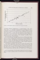

FIGURE 9. Jill Farringdon's sample as scatterplot (with regression line added).
close to either −1 or 1 indicating a strong association (correlation), and r close to
0 indicating a lack of association. Squaring the correlation coefficient (r 2) gives
the portion of variation in the vertical axis that is explained by the horizontal
axis. In this instance, r 2 is .905. That means that 90.5% of the variation we see
in the number of two- and three-letter plus initial-vowel words is explained by
the number of words in the sentence. I had already noted this high degree of
correlation from the visual inspection of this scatterplot; r 2 provides us with a
precise measurement of that correlation.
So for this sample, the relationship between the two variables that Farringdon
wants to measure is highly predictable. And because it is so predictable, it
does
not seem to measure anything that would assist one in trying to
distinguish one
author from another. This high degree of predictability
means that at most 9.5%
of the two- and
three-letter plus initial-vowel words in this sample can be ex-
plained by
something related to Farringdon's so-called "linguistic fingerprint"
that
distinguishes her writing from that of another.
Is this sample representative? The only way to answer that question would
be
to take many samples from various writers, count the relevant words, and
calculate the values of r
2. I did this for three other samples by canonical writers
from different time periods. I selected samples of 31 sentences each from
the
beginnings of these very different works: Samuel Johnson's The Rambler no. 14
(1750), Charlotte Brontë's
Jane Eyre (1847), and Virginia Woolf's To the Lighthouse
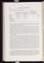
| Author | Average Words per Sentence ± Standard Deviation |
Average 23lw+ivw per Sentence ± Standard Deviation |
Ratio of 23lw+ivw to Total Number of Words per Sentence (slope of regression line) |
r 2 |
| Johnson | 49.6 ± 19.1 | 27.9 ± 11.8 | .58 | .889 |
| Brontë | 31.1 ± 23.2 | 15.4 ± 12.6 | .54 | .972 |
| Woolf | 37.9 ± 38.0 | 19.1 ± 19.4 | .51 | .985 |
| Johnson, Brontë, Woolf, and Farringdon combined (124 sentences total) |
35.2 ± 26.5 | 18.5 ± 14.5 | .54 | .959 |
(1927).[14]
Table 9 presents the compiled data for the samples from these three
works along with a combined dataset that contains all 124 sentences from John-
son, Brontë, Woolf, and Farringdon.
The high values for r
2 show that the primary and almost exclusive factor in
determining the number of two- and three-letter plus initial-vowel words is the
length of the sentence itself. In order to substantiate this point more
fully, one
would have to draw on many more samples. But the evidence I
present here is
quite suggestive. These three writers from three different
centuries have very dif-
ferent styles, as suggested by the very different
average lengths of their sentences.
Despite that important difference, the
similar values of r
2 show that for each of
these three samples, the
correlations between the two measured variables are
extremely strong.
The combined sample of sentences from Johnson, Brontë, Woolf, and Far-
ringdon is even more suggestive. The value of r
2 is again quite high. If one
were to remove sentences
by Johnson from this combined sample, the strength
of the correlation would
not significantly change. The average sentence length
would change, since of
these four writers, Johnson's average sentence length is
the greatest. (Any
casual reader of Johnson's essays knows that his sentences tend
to be
relatively long.) However, the "language-habit" under discussion does not
refer to sentence length by itself, but to the relationship between sentence
length
and two- and three-letter plus initial-vowel words. The information
in table 9
suggests that that relationship (as measured by r
2) will not vary significantly no
matter how many
sentences are removed from the combined sample and re-
gardless of the
authorship of those sentences. At least for these samples, this
"language-habit" fails to distinguish these authors from one another, and a
quantitatively-based attribution method that fails to distinguish between the
writ-
is of no value.
Based on this admittedly limited amount of evidence, I would hypothesize
that the relationship between sentence length and the number of two- and three-
letter plus initial-vowel words is highly predictable, and perhaps
universally so
for non-technical writing in the English language in the
modern period. That
hypothesis is supported by the remarkably similar ratios
between this category
of words and the total number of words for all these
samples. If my hypothesis
is correct, then the relationship is so
predictable that it does not provide a useful
basis for discriminating
between one author and another. To test that hypoth-
esis, one could examine
far more examples than I have to determine whether
or not the r
2 values tend to be .889 or higher. The QSUM proponents have
accumulated an enormous amount of this data, and they could easily perform
the necessary calculations. Doing so is necessary to defend the view that
this
"language-habit" is indeed an individual, unconscious habit, and not a
general
fact of language.
For further discussion of the "least-squares regression line" and the
"correlation
coefficient," see David S. Moore, The
Basic Practice of Statistics (New York: W. H. Freeman,
1995),
111–128. One can calculate the value of r in Microsoft Excel by using
the CORREL
function.
I used the following authoritative editions for these works: Volume 3 of The Yale Edition
of the Works of Samuel Johnson,
ed. W. J. Bate and Albrecht B. Strauss (New Haven: Yale Univ.
Press,
1969), 74–79; Jane Eyre: The Clarendon Edition of
the Novels of the Brontës, ed. Jane Jack and
Margaret
Smith (Oxford: Clarendon Press, 1969), 3–6; and To
the Lighthouse: The Definitive Col-
lected Edition of the Novels of
Virginia Woolf (London: Hogarth Press, 1990), 3–6. I did not
count
the abbreviations "Mr." and "Mrs." as two and three letter
words. For the Jane Eyre sample, I
omitted the
four lines of verse on page 4 because I wanted to examine only prose.
Some Modest Proposals
As I have already suggested, any quantitative attribution method that purports
to be valid must define terms precisely and use statistical concepts in an
appropri-
ate manner. It should also offer a theoretical justification. But
such conditions are
not sufficient. Proponents of quantitative methods must
also rigorously attempt
to falsify their theories. At the hypothetical stage
of testing, the question should
not be "does it work?" but rather "does it
resist all reasonable attempts to make
it fail?" And so I raise these final
points not in relation to QSUM—which can-
not be rescued—but
in regard to other quantitative approaches that have been
offered and will
likely continue to be offered.[15]
One simple falsification test would work as follows. Take the original textual
data set of homogeneous writing, omit a portion from that data set (perhaps
an
entire work), then test the omitted portion against the remaining data
set. Repeat
this test using a different omitted portion and repeat again and
again until every
portion of the data set has been tested. Since this
description might be confusing, I
offer this concrete example. Start with
the complete plays of Shakespeare, exclud-
ing those plays believed to have
been written in collaboration. Process these plays
as necessary, and then
remove Romeo and Juliet from this data set. Now test Romeo
and Juliet against the data set of fully
Shakespearean plays (excluding Romeo and Ju-
liet).
Does the method correctly identify Romeo and Juliet as
Shakespeare's? Re-insert
Romeo and Juliet back into the data set, and remove a
different play to test. Does
the method work for this play? If, after
frequent attempts, the method never fails,
then one has a plausible
hypothesis worth examining. This falsification test has the
added benefit of
determining whether or not a particular method can fail to distin-
guish
between works by the same author that employ radically different styles.
But before going further, one should allow others to verify these falsification
attempts and possibly run further tests. The best way to do this, it seems
to me,
would be to make available the raw texts as well as the data and
formulas on a
publicly accessible website. Then others could download the
tests and examine
the information for themselves.
Proponents of these kinds of methods should also provide their history of
failed attempts. There is no shame in conceiving a method and then finding out
on one's own that it does not work. A description of the process of trial
and er-
ror should actually increase the reader's confidence in the author's
drive to find
a reliable, objective method.
All methods have limitations, and proponents of attribution methods should
acknowledge and describe those limitations. For example: "I have successfully
tested this method on journalistic prose during the first half of the
eighteenth
century, but have found it to be less reliable for poetry or
verse drama." Genre
and time period are obvious limitations, but there are
undoubtedly others. Pro-
ponents should go further by describing the size of
the samples tested. More
importandy, what are the measurements of
reliability? Is this a claim of 99% or
95% certainty? One
benefit of the chi-squared test I mentioned earlier is that it
can calculate
its degree of certainty with precision.
Each method should include a statement of standards for treatment of orthog-
raphy (were texts modernized in any way? were spellings standardized?) as well as
attention to bibliographical matters (which editions were used and
why?).[16]
Proponents of attribution methods must also distinguish between those that
reliably disprove authorship versus those that assert it. One can easily imagine a
method that can show that a particular author did not write a particular
work,
but cannot show with any degree of certainty that a different author
did write
the work.
Finally, I would make a plea that proponents separate their arguments in
support of the method from its application in particular cases. That is, propo-
nents should first independendy publish an account that describes the method
and its limitations as well as how it responds to known and accepted cases
of
authorship. This step should give the scholarly community an opportunity
to
examine the method and respond. Only after a reasonable time to allow for
this
exchange should proponents begin to offer attributions (or
de-attributions) of
particular examples. I hope that this delay would
decrease irresponsible claims
of authorship.
For a useful survey of other quantitative approaches and a judicious
assessment of the
potential pitfalls and rewards of this burgeoning
subfield, see Harold Love, Attributing Author-
ship, 132–162.
For a thorough discussion of these and related concerns, see Joseph Rudman,
"Un-
editing, De-Editing, and Editing in Non-traditional Authorship
Attribution Studies: With an
Emphasis on the Canon of Daniel Defoe,"
Papers of the Bibliographical Society of America
99 (2005):
5–36.
I am grateful to the following people who gave me advice and encouragement on
this
article: Amy L. Blair, Haruki Toyama, Jodi Melamed, James Woolley,
and Maya C. Gibson.
I am especially grateful to my father, Zaven A.
Karian, who advised me on various statistical
concepts. I alone am
responsible for any errors in this article.
For a useful collection of essays on the broad subject of attribution in
literary study,
see Evidence for Authorship: Essays on
Problems of Attribution, ed. David V. Erdman and Ephim G.
Fogel
(Ithaca: Cornell Univ. Press, 1966). Though more than forty years old, this
collection
remains quite valuable. For a more recent discussion, see
Harold Love, Attributing Authorship:
An
Introduction (Cambridge: Cambridge Univ. Press, 2002).
Here and throughout this paper I use the abbreviation QSUM to refer only to
the attribution theory under discussion. The theory's proponents use both
"QSUM" and
"cusum analysis" interchangeably. As I discuss later,
cumulative sum analysis (often abbrevi-
ated CUSUM) can also refer to a
statistical technique derived from another field.
| Studies in bibliography | ||